Developing Customized Branch-&-Cut algorithms

This chapter discusses some features of Python-MIP that allow the development of improved Branch-&-Cut algorithms by linking application specific routines to the generic algorithm included in the solver engine. We start providing an introduction to cutting planes and cut separation routines in the next section, following with a section describing how these routines can be embedded in the Branch-&-Cut solver engine using the generic cut callbacks of Python-MIP.

Cutting Planes

In many applications there are strong formulations that may include an exponential number of constraints. These formulations cannot be direct handled by the MIP Solver: entering all these constraints at once is usually not practical, except for very small instances. In the Cutting Planes [Dantz54] method the LP relaxation is solved and only constraints which are violated are inserted. The model is re-optimized and at each iteration a stronger formulation is obtained until no more violated inequalities are found. The problem of discovering which are the missing violated constraints is also an optimization problem (finding the most violated inequality) and it is called the Separation Problem.

As an example, consider the Traveling Salesman Problem. The compact formulation (tsp-label) is a weak formulation: dual bounds produced at the root node of the search tree are distant from the optimal solution cost and improving these bounds requires a potentially intractable number of branchings. In this case, the culprit are the sub-tour elimination constraints linking variables \(x\) and \(y\). A much stronger TSP formulation can be written as follows: consider a graph \(G=(N,A)\) where \(N\) is the set of nodes and \(A\) is the set of directed edges with associated traveling costs \(c_a \in A\). Selection of arcs is done with binary variables \(x_a \,\,\, \forall a \in A\). Consider also that edges arriving and leaving a node \(n\) are indicated in \(A^+_n\) and \(A^-_n\), respectively. The complete formulation follows:

\[\begin{split} \textrm{Minimize:} & \\ & \sum_{a \in A} c_a\ldotp x_a \\ \textrm{Subject to:} & \\ & \sum_{a \in A^+_n} x_a = 1 \,\,\, \forall n \in N \\ & \sum_{a \in A^-_n} x_a = 1 \,\,\, \forall n \in N \\ & \sum_{(i,j) \in A : i\in S \land j \in S} x_{(i,j)} \leq |S|-1 \,\,\, \forall \,\, S \subset I \\ & x_a \in \{0,1\} \,\,\, \forall a \in A\end{split}\]

The third constraints are sub-tour elimination constraints. Since these constraints are stated for every subset of nodes, the number of these constraints is \(O(2^{|N|})\). These are the constraints that will be separated by our cutting pane algorithm. As an example, consider the following graph:

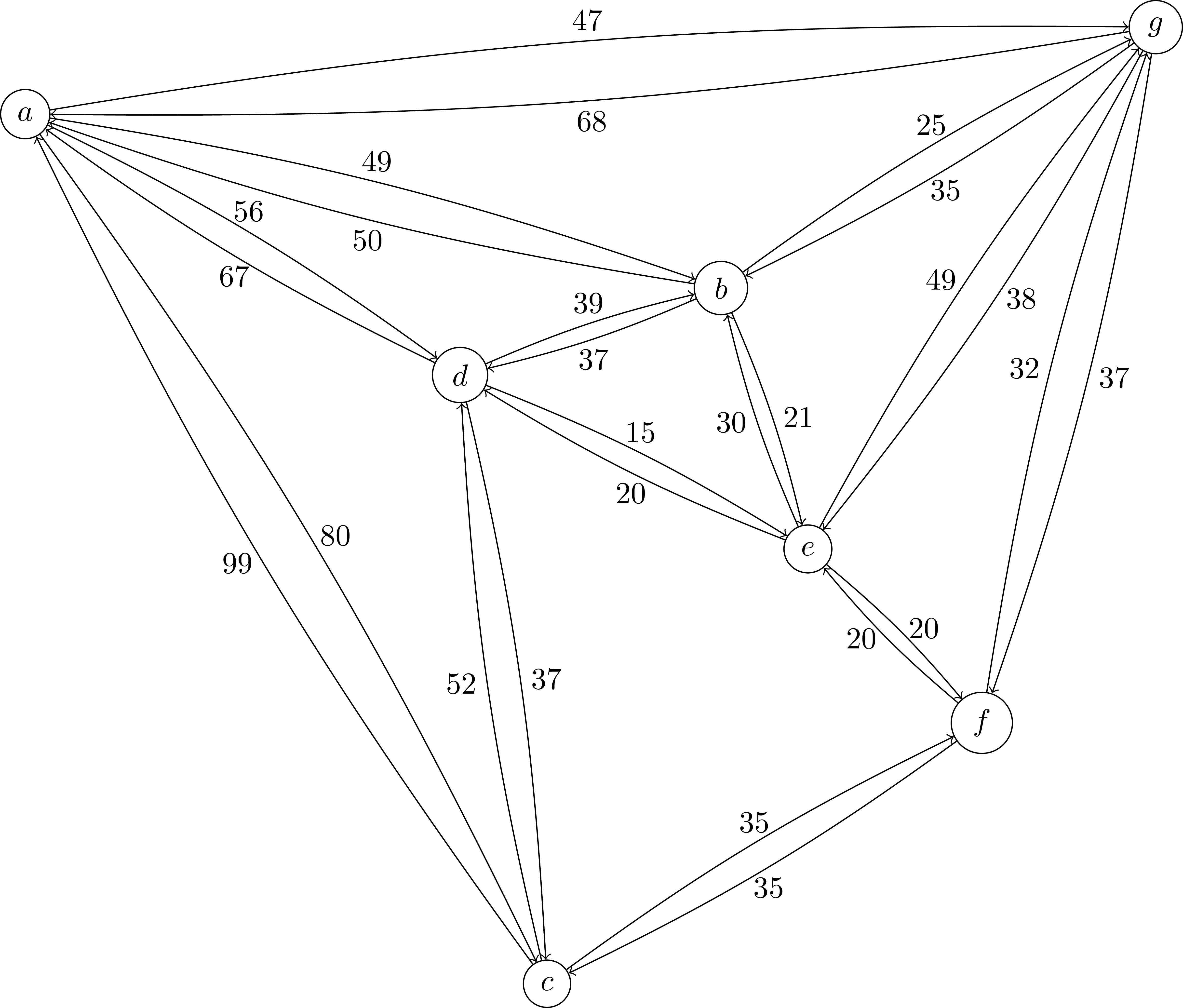
The optimal LP relaxation of the previous formulation without the sub-tour elimination constraints has cost 237:

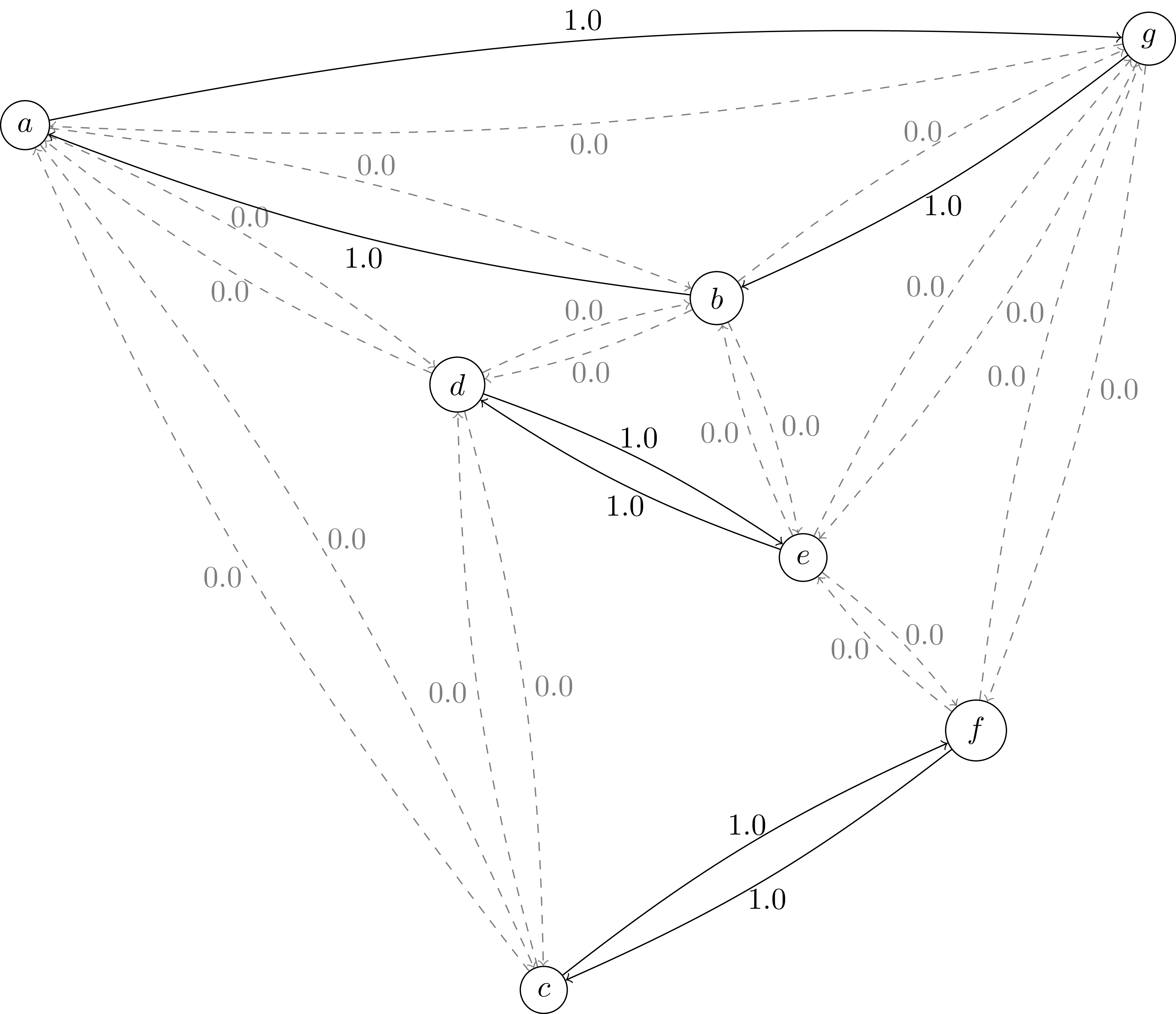
As it can be seen, there are tree disconnected sub-tours. Two of these include only two nodes. Forbidding sub-tours of size 2 is quite easy: in this case we only need to include the additional constraints: \(x_{(d,e)}+x_{(e,d)}\leq 1\) and \(x_{(c,f)}+x_{(f,c)}\leq 1\).

Optimizing with these two additional constraints the objective value increases to 244 and the following new solution is generated:

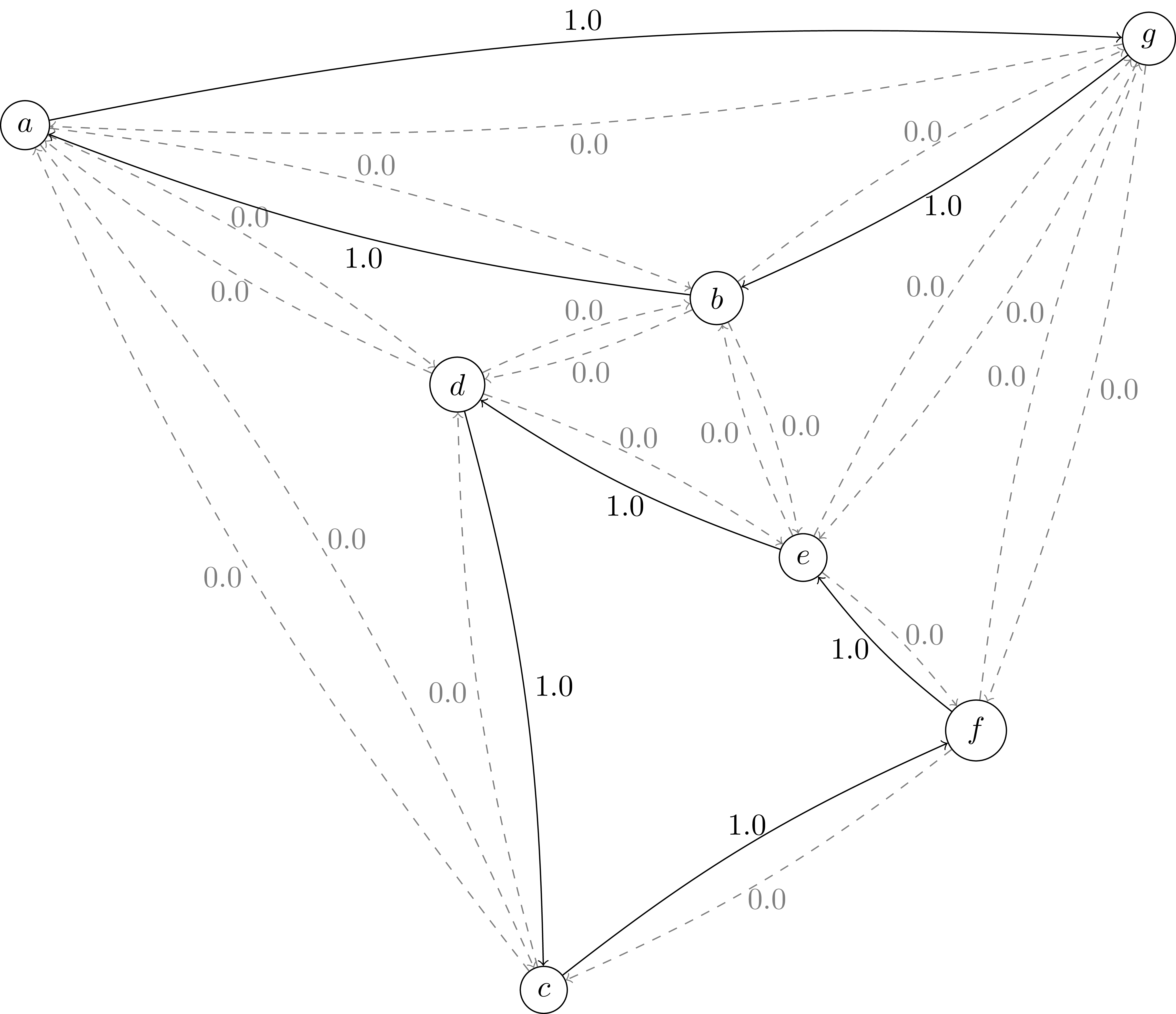
Now there are sub-tours of size 3 and 4. Let’s consider the sub-tour defined by nodes \(S=\{a,b,g\}\). The valid inequality for \(S\) is: \(x_{(a,g)} + x_{(g,a)} + x_{(a,b)} + x_{(b,a)} + x_{(b,g)} + x_{(g,b)} \leq 2\). Adding this cut to our model increases the objective value to 261, a significant improvement. In our example, the visual identification of the isolated subset is easy, but how to automatically identify these subsets efficiently in the general case ? Isolated subsets can be identified when a cut is found in the graph defined by arcs active in the unfeasible solution. To identify the most isolated subsets we just have to solve the Minimum cut problem in graphs. In python you can use the networkx min-cut module. The following code implements a cutting plane algorithm for the asymmetric traveling salesman problem:

A pure cutting-planes approach for the Traveling Salesman Problem (examples/cutting_planes.py)

from itertools import product
from networkx import minimum_cut, DiGraph
from mip import Model, xsum, BINARY, OptimizationStatus, CutType

N = ["a", "b", "c", "d", "e", "f", "g"]
A = { ("a", "d"): 56, ("d", "a"): 67, ("a", "b"): 49, ("b", "a"): 50,
      ("f", "c"): 35, ("g", "b"): 35, ("g", "b"): 35, ("b", "g"): 25,
      ("a", "c"): 80, ("c", "a"): 99, ("e", "f"): 20, ("f", "e"): 20,
      ("g", "e"): 38, ("e", "g"): 49, ("g", "f"): 37, ("f", "g"): 32,
      ("b", "e"): 21, ("e", "b"): 30, ("a", "g"): 47, ("g", "a"): 68,
      ("d", "c"): 37, ("c", "d"): 52, ("d", "e"): 15, ("e", "d"): 20,
      ("d", "b"): 39, ("b", "d"): 37, ("c", "f"): 35, }
Aout = {n: [a for a in A if a[0] == n] for n in N}
Ain = {n: [a for a in A if a[1] == n] for n in N}

m = Model()
x = {a: m.add_var(name="x({},{})".format(a[0], a[1]), var_type=BINARY) for a in A}

m.objective = xsum(c * x[a] for a, c in A.items())

for n in N:
    m += xsum(x[a] for a in Aout[n]) == 1, "out({})".format(n)
    m += xsum(x[a] for a in Ain[n]) == 1, "in({})".format(n)

newConstraints = True

while newConstraints:
    m.optimize(relax=True)
    print("status: {} objective value : {}".format(m.status, m.objective_value))

    G = DiGraph()
    for a in A:
        G.add_edge(a[0], a[1], capacity=x[a].x)

    newConstraints = False
    for (n1, n2) in [(i, j) for (i, j) in product(N, N) if i != j]:
        cut_value, (S, NS) = minimum_cut(G, n1, n2)
        if cut_value <= 0.99:
            m += (xsum(x[a] for a in A if (a[0] in S and a[1] in S)) <= len(S) - 1)
            newConstraints = True
    if not newConstraints and m.solver_name.lower() == "cbc":
        cp = m.generate_cuts([CutType.GOMORY, CutType.MIR, 
                              CutType.ZERO_HALF, CutType.KNAPSACK_COVER])
        if cp.cuts:
            m += cp
            newConstraints = True

Lines 6-13 are the input data. Nodes are labeled with letters in a list N and a dictionary A is used to store the weighted directed graph. Lines 14 and 15 store output and input arcs per node. The mapping of binary variables \(x_a\) to arcs is made also using a dictionary in line 18. Line 20 sets the objective function and the following tree lines include constraints enforcing one entering and one leaving arc to be selected for each node. Line 29 will only solve the LP relaxation and the separation routine can be executed. Our separation routine is executed for each pair or nodes at line 38 and whenever a disconnected subset is found the violated inequality is generated and included at line 40. The process repeats while new violated inequalities are generated.

Python-MIP also supports the automatic generation of cutting planes, i.e., cutting planes that can be generated for any model just considering integrality constraints. Line 43 triggers the generation of these cutting planes with the method generate_cuts() when our sub-tour elimination procedure does not finds violated sub-tour elimination inequalities anymore.

Cut Callback

The cutting plane method has some limitations: even though the first rounds of cuts improve significantly the lower bound, the overall number of iterations needed to obtain the optimal integer solution may be too large. Better results can be obtained with the Branch-&-Cut algorithm, where cut generation is combined with branching. If you have an algorithm like the one included in the previous Section to separate inequalities for your application you can combine it with the complete BC algorithm implemented in the solver engine using callbacks. Cut generation callbacks (CGC) are called at each node of the search tree where a fractional solution is found. Cuts are generated in the callback and returned to the MIP solver engine which adds these cuts to the Cut Pool. These cuts are merged with the cuts generated with the solver builtin cut generators and a subset of these cuts is included to the LP relaxation model. Please note that in the Branch-&-Cut algorithm context cuts are optional components and only those that are classified as good cuts by the solver engine will be accepted, i.e., cuts that are too dense and/or have a small violation could be discarded, since the cost of solving a much larger linear program may not be worth the resulting bound improvement.

When using cut callbacks be sure that cuts are used only to improve the LP relaxation but not to define feasible solutions, which need to be defined by the initial formulation. In other words, the initial model without cuts may be weak but needs to be complete 1. In the case of TSP, we can include the weak sub-tour elimination constraints presented in tsp-label in the initial model and then add the stronger sub-tour elimination constraints presented in the previous section as cuts.

In Python-MIP, CGC are implemented extending the ConstrsGenerator class. The following example implements the previous cut separation algorithm as a ConstrsGenerator class and includes it as a cut generator for the branch-and-cut solver engine. The method that needs to be implemented in this class is the generate_constrs() procedure. This method receives as parameter the object model of type Model. This object must be used to query the fractional values of the model vars, using the x property. Other model properties can be queried, such as the problem constraints (constrs). Please note that, depending on which solver engine you use, some variables/constraints from the original model may have been removed in the pre-processing phase. Thus, direct references to the original problem variables may be invalid. The method translate() (line 15) translates references of variables from the original model to references of variables in the model received in the callback procedure. Whenever a violated inequality is discovered, it can be added to the model using the += operator (line 31). In our example, we temporarily store the generated cuts in a CutPool object (line 25) to discard repeated cuts that eventually are found.

Branch-and-cut for the traveling salesman problem (examples/tsp-cuts.py)

from typing import List, Tuple
from random import seed, randint
from itertools import product
from math import sqrt
import networkx as nx
from mip import Model, xsum, BINARY, minimize, ConstrsGenerator, CutPool


class SubTourCutGenerator(ConstrsGenerator):
    """Class to generate cutting planes for the TSP"""
    def __init__(self, Fl: List[Tuple[int, int]], x_, V_):
        self.F, self.x, self.V = Fl, x_, V_

    def generate_constrs(self, model: Model, depth: int = 0, npass: int = 0):
        xf, V_, cp, G = model.translate(self.x), self.V, CutPool(), nx.DiGraph()
        for (u, v) in [(k, l) for (k, l) in product(V_, V_) if k != l and xf[k][l]]:
            G.add_edge(u, v, capacity=xf[u][v].x)
        for (u, v) in F:
            val, (S, NS) = nx.minimum_cut(G, u, v)
            if val <= 0.99:
                aInS = [(xf[i][j], xf[i][j].x)
                        for (i, j) in product(V_, V_) if i != j and xf[i][j] and i in S and j in S]
                if sum(f for v, f in aInS) >= (len(S)-1)+1e-4:
                    cut = xsum(1.0*v for v, fm in aInS) <= len(S)-1
                    cp.add(cut)
                    if len(cp.cuts) > 256:
                        for cut in cp.cuts:
                            model += cut
                        return
        for cut in cp.cuts:
            model += cut


n = 30  # number of points
V = set(range(n))
seed(0)
p = [(randint(1, 100), randint(1, 100)) for i in V]  # coordinates
Arcs = [(i, j) for (i, j) in product(V, V) if i != j]

# distance matrix
c = [[round(sqrt((p[i][0]-p[j][0])**2 + (p[i][1]-p[j][1])**2)) for j in V] for i in V]

model = Model()

# binary variables indicating if arc (i,j) is used on the route or not
x = [[model.add_var(var_type=BINARY) for j in V] for i in V]

# continuous variable to prevent subtours: each city will have a
# different sequential id in the planned route except the first one
y = [model.add_var() for i in V]

# objective function: minimize the distance
model.objective = minimize(xsum(c[i][j]*x[i][j] for (i, j) in Arcs))

# constraint : leave each city only once
for i in V:
    model += xsum(x[i][j] for j in V - {i}) == 1

# constraint : enter each city only once
for i in V:
    model += xsum(x[j][i] for j in V - {i}) == 1

# (weak) subtour elimination
# subtour elimination
for (i, j) in product(V - {0}, V - {0}):
    if i != j:
        model += y[i] - (n+1)*x[i][j] >= y[j]-n

# no subtours of size 2
for (i, j) in Arcs:
    model += x[i][j] + x[j][i] <= 1

# computing farthest point for each point, these will be checked first for
# isolated subtours
F, G = [], nx.DiGraph()
for (i, j) in Arcs:
    G.add_edge(i, j, weight=c[i][j])
for i in V:
    P, D = nx.dijkstra_predecessor_and_distance(G, source=i)
    DS = list(D.items())
    DS.sort(key=lambda x: x[1])
    F.append((i, DS[-1][0]))

model.cuts_generator = SubTourCutGenerator(F, x, V)
model.optimize()

print('status: %s route length %g' % (model.status, model.objective_value))

Lazy Constraints

Python-MIP also supports the use of constraint generators to produce lazy constraints. Lazy constraints are dynamically generated, just as cutting planes, with the difference that lazy constraints are also applied to integer solutions. They should be used when the initial formulation is incomplete. In the case of our previous TSP example, this approach allow us to use in the initial formulation only the degree constraints and add all required sub-tour elimination constraints on demand. Auxiliary variables \(y\) would also not be necessary. The lazy constraints TSP example is exactly as the cut generator callback example with the difference that, besides starting with a smaller formulation, we have to inform that the constraint generator will be used to generate lazy constraints using the model property lazy_constrs_generator.

...
model.cuts_generator = SubTourCutGenerator(F, x, V)
model.lazy_constrs_generator = SubTourCutGenerator(F, x, V)
model.optimize()
...

Providing initial feasible solutions

The Branch-&-Cut algorithm usually executes faster with the availability of an integer feasible solution: an upper bound for the solution cost improves its ability of pruning branches in the search tree and this solution is also used in local search MIP heuristics. MIP solvers employ several heuristics for the automatically production of these solutions but they do not always succeed.

If you have some problem specific heuristic which can produce an initial feasible solution for your application then you can inform this solution to the MIP solver using the start model property. Let’s consider our TSP application (tsp-label). If the graph is complete, i.e. distances are available for each pair of cities, then any permutation \(\Pi=(\pi_1,\ldots,\pi_n)\) of the cities \(N\) can be used as an initial feasible solution. This solution has exactly \(|N|\) \(x\) variables equal to one indicating the selected arcs: \(((\pi_1,\pi_2), (\pi_2,\pi_3), \ldots, (\pi_{n-1},\pi_{n}), (\pi_{n},\pi_{1}))\). Even though this solution is obvious for the modeler, which knows that binary variables of this model refer to arcs in a TSP graph, this solution is not obvious for the MIP solver, which only sees variables and a constraint matrix. The following example enters an initial random permutation of cities as initial feasible solution for our TSP example, considering an instance with n cities, and a model model with references to variables stored in a matrix x[0,...,n-1][0,..,n-1]:

from random import shuffle
S=[i for i in range(n)]
shuffle(S)
model.start = [(x[S[k-1]][S[k]], 1.0) for k in range(n)]

The previous example can be integrated in our TSP example (tsp-label) by inserting these lines before the model.optimize() call. Initial feasible solutions are informed in a list (line 4) of (var, value) pairs. Please note that only the original non-zero problem variables need to be informed, i.e., the solver will automatically compute the values of the auxiliary \(y\) variables which are used only to eliminate sub-tours.

Footnotes

1

If you want to initally enter an incomplete formulation than see the next sub-section on Lazy-Constraints.